Examples
We present here three examples of analysis using SMARTPOP. The bash scripts and R code can be downloaded here.
More examples are available in the original paper: SMARTPOP: inferring the impact of social dynamics on genetic diversity through high speed simulations by Guillot and Cox, BMC Bioinformatics 2014 15:175.
Equilibrium state of diversity depending on the population size
Comparing the dynamics of diversity between monogamous and polygamous populations
Dynamics of diversity in a population that grew before reaching a stable population size.
Equilibrium state of diversity depending on the population size
In this example, we run 500 simulations (-nsimu 500) with a population of 100 individuals (-p 100) having a polygamous mating system (-mat 2). We measure diversity estimators for the population after a long run when the population has reached equilibrium (-t 10000). We check the diversity on a sample of 50 individuals (-sample 20). The output will be named example1 (-o example1), and includes the header for the analysis (-header)
./smartpop -p 100 -mat 2 -t 10000 -sample 50 -header -o example1
To produce datasets for higher population sizes, we just repeat the same command with the desired population size. We will append the results to the same file. The header should not be added each time, so we must get remove the -header flag.
./smartpop -p 500 -mat 2 -t 10000 -sample 50 -o example1
./smartpop -p 1000 -mat 2 -t 10000 -sample 50 -o example1
Using an R script, we can look at the diversity at equilibrium depending on the population size.

Simulated θπ depending on the population size.
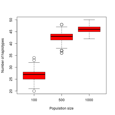
Simulated number of haplotypes depending on the population size.
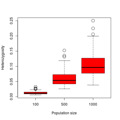
Simulated heterozygosity depending on the population size.
Comparing the dynamics of diversity patterns between monogamy and polygamy
In this example, we run 500 simulations (-nsimu 500) with a population of 100 individuals (-p 100) having a monogamous system (-mat 1) with no sibling alliance (-noSib). This simulation uses a burn-in phase to first increase the population diversity until θπ reaches 25 (-burnin 25). We then follow different estimators in the population through time. The diversity is checked on a sample of 20 individuals (-sample 20) every 5 generations (-t 5), 50 successive times (-nstep 50). The output files will be named example2_mono (-o example2_mono) and include the header for the analysis (-header).
The complete command line to produce the monogamous simulations is:
./smartpop -p 100 -nsimu 500 -mat 1 -sample 20 -noSib -t 5 -nstep 50 -o example2_mono -header
The complete command line to produce the polygamous simulations is:
./smartpop -p 100 -nsimu 500 -mat 2 -sample 20 -noSib -t 5 -nstep 50 -o example2_poly -header
This will create the following files:
- example2_monoMt: Estimators on simulated mtDNA through time under monogamy.
- example2_monoX: Estimators on simulated X chromosome through time under monogamy.
- example2_monoY: Estimators on simulated Y chromosome through time under monogamy.
- example2_monoA: Estimators on simulated autosomes through time under monogamy.
- example2_polyMt: Estimators on simulated mtDNA through time under polygamy.
- example2_polyX: Estimators on simulated X chromosome through time under polygamy.
- example2_polyY: Estimators on simulated Y chromosome through time under polygamy.
- example2_polyA: Estimators on simulated autosomes through time under polygamy.
Those outputs can be analyzed using R (cf. example2.R).
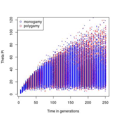
θπ through time. Red points represent monogamous populations, blue points represent polygamous populations.
It is more readable to measure the mean of simulations having the same mating system at the same time point.
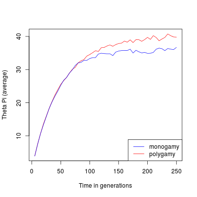
Average θπ through time. The red line represents monogamous populations, the blue line represents polygamous populations.
It is interesting to follow the number of haplotypes on the same simulation set.
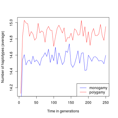
Average number of haplotypes through time. The red line represents monogamous populations, the blue line represents polygamous populations.
With this example, looking at average values you can see that the mating system introduce a difference in the population genetic diversity using both estimators. This difference is however quite small. The scatter plot show a large variance between simulations which makes the difference between monogamy and polygamy non significant.
Dynamics of diversity in a population that grew before reaching a stable population size.
In this example, we run 500 simulations (-nsimu 500) with a population of 100 individuals (-p 100) at equilibrium, growing linearly to 200 individuals in 50 generations (thus gaining two individuals per generation for 50 generations), then staying constant for 5000 generations.
To simulate such complex scenario, we must divide the run in three phases, each phase having a unique set of parameters. In this case we will first simulate the 100 individuals at equilibrium (i.e. evolving for a long time). The second phase will simulate the growth. The last phase will simulate the final 5000 generations with constant population size. The only trick to collate these scenarios is to save the populations and reload them using the flags -save and -load. We can also save the evolution of the mitochondrial DNA from these simulations from the start of the growth, sampling 50 individuals every 5 years. To look at mtDNA only, it is faster to use the flag -mtdiv. The output will be saved under the name example3.
./smartpop -p 100 -t 20 -nstep 50 -sample 50 -save phase1 -nbLociX 0 -sizeY 0 -nbLociA 0 -o example3 -header -nsimu 500
./smartpop -t 5 -nstep 10 -sample 50 -o example3 -demog 2 1 0 -load phase1 -save phase2 -mtdiv -nsimu 500
./smartpop -t 10 -nstep 100 -sample 50 -o example3 -load phase2 -mtdiv -nsimu 500
The output file example3_mt_div.txt can be analyzed with R to produce the following plots.
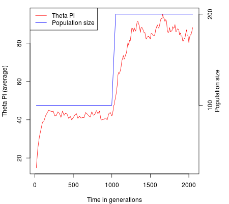
The red line represents the average θπ through time (left axis). The blue line represents the population size through time (right axis).
It can be interesting to follow the number of haplotypes in the same simulation set.
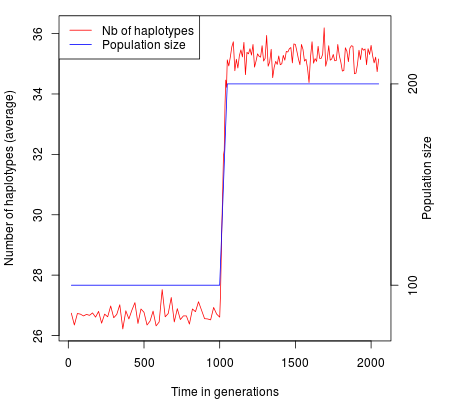
The red line represents the average number of haplotypes through time (left axis). The blue line represents the population size through time (right axis).
This example show the disequilibrium in diversity introduced by a very small growth (2 individuals / year). Although the number of haplotypes settle quite fast when the population size becomes stable, the mean pairwise distance, illustrated by $\theta_\pi$ takes hundreds of generation, i.e. thousands of years, before reaching its higher value.
